Insolation vs. Temperature

March 19, 2014

Some time ago I mentioned the phase difference between local temperature and insolation, trying to find the warmest day of the year in the given location (somewhere in here, http://climateaudit.org/2011/09/13/some-simple-questions/ cant locate the exact link now update: http://climateaudit.org/2011/09/28/monthly-centering-and-climate-sensitivity ). It is well known that the input to the system (solar insolation) peaks about one month before the output (local temperature). Being too lazy to read the relevant literature (ref 1-3 etc.) I built a simple recursive model for local temperature
[tex]t(k)=t(k-1)+As(t)-Bt(k-1)^4+Ct_2(k-1)^4[/tex],
where t is local temperature, s(t) insolation, t_2 temperature of a large mass nearby that location, k time index and A,B,C parameters that describe local conditions. This extra mass was needed to achieve satisfactory phase response, with similar equation:
[tex]t_2(k)=t_2(k-1)+Ds(t)-Et_2(k-1)^4+Ft(k-1)^4[/tex].
For solar data, I built a Matlab model of Earth-Sun system with orbital parameters from (4-6) and checked from nautical almanac (7) that the Sun position agrees with the model for year 2011. Basic checks to see if solar data is ok:
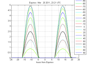
eq1
Figure 1. Insolation at Greenwich meridian during Mar 2011 Equinox, time from (4), (per latitude, time resolution 1 hour).
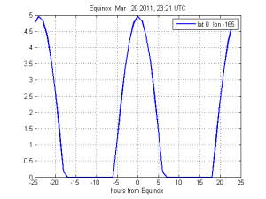
eq2
Figure 2. Insolation at 165 West longitude, 0 latitude, during Mar 2011 Equinox, time from (4), (time resolution 1 hour).
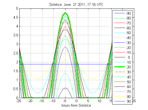
solst1
Figure 3. Insolation at Greenwich meridian during June 2011 Solstice, time from (4), (per latitude, time resolution 1 hour).

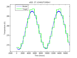
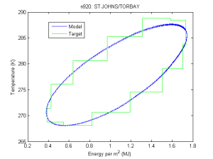
Finding the parameters was then just a minimization problem, using Jones 90 data as reference for the t(k). Jones data is monthly data so monthly means of t(k) were used for minimization. Result from one randomly picked station shown in the figures below.
blog1
Fig 4. Model output versus measured temperatures
blog2
Fig 5. Insolation vs. temperature
 

Data in here : http://www.climateaudit.info/data/uc/modeldata920.txt

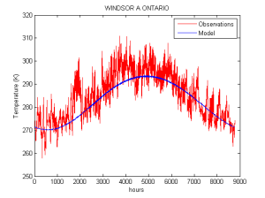
For some stations hourly temperatures are available (8). I took Windsor Ontario as an example:
blog_windsor
Fig 6. Windsor hourly temperature for 2012 vs. model
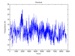
blog_residual
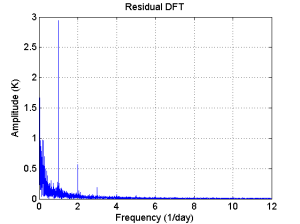
Fig 7. Windsor residual

blog_residual_dft
Fig 8. Windsor residual in frequency domain

Data in here: http://www.climateaudit.info/data/uc/WindsorData.txt

The mean of the residual is 2.6 C, and standard deviation 5.4 C. AR(1) lag-1 coefficient is 0.98, but local Whittle estimate for memory parameter d is 0.66 so one could say the residual represents some complex fractional stochastic process ( as weather often is convenient to describe, only in climatic scales miracles happen and neat AR1 processes only remain for GMT trend analysis (9)). Diurnal variation is clearly damped (see Fig. 8), so we just state that this model represents temperature 10 cm below ground or so ;)

Is this model useful? Don’t know yet. Next step would be to add white noise to s(t) and find out if the model can produce local time series with similar autocorrelation properties as real observations. Or see if changes in insolation agree with the results that physical climate models give. Or generate one Kalman filter for each station and see if they together can predict GMT anomaly. But the main reason was just to try to find one way to explain the phase differences, and that task was accomplished. There is quite a lot of parameters to fit, but if I leave constant part out (the model now works with Kelvins that agree with reality) I get similar results with an IIR filter that has 3 parameters per location.

1. Rohde et. al 2013, Appendix to Berkeley Earth Temperature Averaging Process:Details of Mathematical and Statistical Methods
2. North et. al, Differences between Seasonal and Mean Annual Energy Balance Model Calculations of Climate and Climate Sensitivity, Journal of the Atmospheric Sciences, 1979
3. Laskar et. al, A long-term numerical solution for the insolation quantities of the Earth, Astronomy and Astrophysics 2004
4. http://aa.usno.navy.mil/data/docs/EarthSeasons.php
5. http://aa.usno.navy.mil/faq/
6. http://nssdc.gsfc.nasa.gov/planetary/factsheet/earthfact.html
7. http://www.erikdeman.de/html/sail003a.htm
8. http://climate.weather.gc.ca/
9. http://climateaudit.org/2007/07/04/the-new-ipcc-test-for-long-term-persistence/
First Ever Successful Prediction of GMT! 3 Years Done!

August 30, 2011

Sorry about the title.

My prediction of the GMT, HadCRUT (NH+SH)/2 monthly time series is now three years old. Before checking the results I would like to list some important requirements for predictions of this kind:

1) Predictions need to include prediction intervals. Predictions without prediction intervals (or such indications of confidence) are useless.

2) There has to be a reasonable mathematical or physical model behind the prediction

Note that one cannot succeed in 1 without having the requirement 2 fulfilled.

3) Prediction intervals shouldn’t be too wide. Floor to ceiling approach is too easy. The true value should pass the upper or lower limit from time to time (as the selected confidence level suggests).

4) If your prediction clearly fails, let it go. Do not move the goalposts after the fact.

Here is the result so far:

Prediction

One could claim that this is a failed prediction, as there are so few values below the prediction mean. I could perform a statistical test to check it (MC runs indicate that it is ok), but I’ll do it later. Details about this prediction (requirement 2) are to be published later.

The prediction was originally presented in here ( http://climateaudit.org/2008/07/29/koutsoyiannis-et-al-2008-on-the-credibility-of-climate-predictions/ )

The Trick Timeline

February 26, 2010

Date: 16 Nov 1999, Phil


I’ve just completed Mike’s Nature trick of adding in the real temps
to each series for the last 20 years (ie from 1981 onwards) amd from
1961 for Keith’s to hide the decline.

Date: 22 Dec 2004, mike

No researchers in this field have ever, to our knowledge, “grafted the thermometer record onto” any reconstruction. It is somewhat disappointing to find this specious claim (which we usually find originating from industry-funded climate disinformation websites) appearing in this forum. Most proxy reconstructions end somewhere around 1980, for the reasons discussed above. Often, as in the comparisons we show on this site, the instrumental record (which extends to present) is shown along with the reconstructions, and clearly distinguished from them (e.g. highlighted in red as here).

Date: 6 May 2009, UC


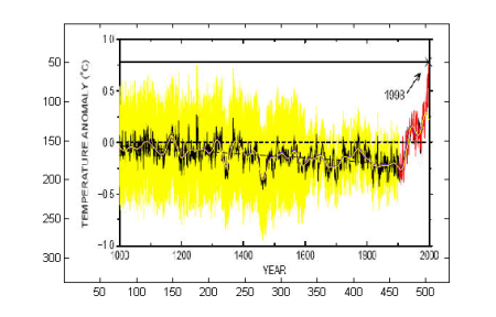
Let’s see; I think this is made by padding with zeros, but 1981-1998 instrumental is grafted onto reconstruction:

(larger image here )

I used Mann’s lowpass.m , modified to pad with zeros instead of mean of the data,

out=lowpass0(data,1/40,0,0);

mbh99smooths

Original CA link

Backup

Date: 20 Nov 2009, UC

“I’ve just completed Mike’s Nature trick of adding in the real temps
to each series for the last 20 years (ie from 1981 onwards) amd from
1961 for Keith’s to hide the decline”

Is this about the MBH99 smooth ?

http://www.climateaudit.org/?p=1553#comment-340175

http://www.climateaudit.org/?p=1553#comment-340207

Date: 20 Nov 2009, gavin

[Response: This has nothing to do with Mann’s Nature article. The 50-year smooth in figure 5b is only of the reconstruction, not the instrumental data. – gavin]

Date: 21 Nov 2009, gavin

And it remains unclear why this was described as Mann’s Nature trick since no such effect is seen in Mike’s paper in any case. – gavin]

Date: 22 Nov 2009, mike

In some earlier work though (Mann et al, 1999), the boundary condition for the smoothed curve (at 1980) was determined by padding with the mean of the subsequent data (taken from the instrumental record).

Date: 24 Nov 2009, CRU

To produce temperature series that were completely up-to-date (i.e. through to 1999) it was necessary to combine the temperature reconstructions with the instrumental record, because the temperature reconstructions from proxy data ended many years earlier whereas the instrumental record is updated every month. The use of the word “trick” was not intended to imply any deception.

Date: 25 Nov 2009, Jean S

UC has corrected me on the fact that adding the instrumental series to the proxy data prior smoothing was used already in MBH98 (Figure 5b), so, unlike I claimed in #66, “Mike’s Nature trick” is NOT a misnomer.

Date: 25 Nov 2009, UC

..and here’s instrumental (81-95)+zero padded Fig 5b smooth (red):

mbh98smooths

Original CA link

Backup

Date: 1 Apr 2010, UC

April Fools, here’s the turn-key(*) code

(*) after you download the two files , http://www.climateaudit.info/wp-content/uploads/2009/11/mbhsmooths1.txt and https://uc00.files.wordpress.com/2010/05/mbh985b.png

Some Interesting Figures (II)

December 21, 2008

Continuation of Figures , mostly these posts serve as pointers to myself, but some may find these useful. Pictures you wont see at RC.

  1. Mann et al 2008
  2. Read the rest of this entry »

Predicting Temperatures

December 15, 2008

On August 27th 08, before August HadCRUT nh+sh temperature was available, I posted this prediction ( http://signals.auditblogs.com/files/2008/08/gmt_pred.txt (dead link, file in here now) at CA:

After four months, it is good to check how well the simple half-integrated-white-noise model is doing. Predictions for these 4 months were

Year        Month     -2 sigma     Predict.     +2 sigma
2008              8       0.15206     0.34864      0.54521
2008              9       0.1141       0.33388      0.55365
2008             10      0.094005    0.32581      0.55762
2008             11      0.080432    0.32024      0.56005

and observations today 15th Dec 08 on HadCRU website are the following:

2008/08 0.396
2008/09 0.374
2008/10 0.438
2008/11 0.387

Here’s how these fit to the original figure:

gmt_pred_upd.png

The model is doing quite good work. I’ll tell you when we reach the upper bound of the prediction interval. And after temperatures go permanently above that bound, AGW kicks this model to the trash can.

Update March 2010


Feb 2010 value is available, I have so far predicted 19 months quite successfully. Let’s see when the model breaks down..

feb10te:

Moore et al. 2005

September 25, 2008

I originally planned to write a long post about signals and noise, but I guess it is better to focus on tiny details and write a book later.  Article New Tools for Analyzing Time
Series Relationships and Trends
by J. C. Moore, A. Grinsted, and S. Jevrejeva (Eos, Vol. 86, No. 24, 14 June 2005) got some attention in David Stockwell’s blog,  http://landshape.org/enm/rahmstorf-et-al-2007-ipcc-error/ . Very interesting article, but I’m afraid there’s something wrong with statements as

A wise choice of embedding dimension can be made with a priori insight or perhaps more commonly may be found by simply playing with the data.

Specially, Figure 3. of that article caught my eye:

Read the rest of this entry »

Hockeystick for Matlab

July 1, 2008

Here’s the version 1.1: hockeystick1.txt

UPD Jan 2010: change

urlwrite(‘http://www.climateaudit.org/data/mbh99/proxy.txt’,’proxy.txt’)

to

urlwrite(‘http://www.climateaudit.info/data/mbh99/proxy.txt’,’proxy.txt’) , or use the new code page

Some notes:

  • Download to empty folder and rename to hockeystick.m
  • Program downloads necessary data from the web (once), uses urlwrite.m (newish Matlab needed)
  • It’s a script
  • Shows what PC1_fixed does
  • Only one file is downloaded from CA (AD1000 proxies), sorry RC, but I don’t know where to find morc014 elsewhere..
  • Pl. tell me if it works or not, uc_edit at yahoo.com !

Updated to Ver 1.1, added cooling trends:

fig1.1.png

Some Interesting Figures

January 3, 2008

While discussing at CA, I’ve made some figures that are spread around CA posts. Here’s a collection of the interesting ones, along with link to CA post in question. All those seem to be related to Dr. Mann’s work. I wonder why..

  1. Re-scaling the Mann and Jones 2003 PC1
  2. Read the rest of this entry »

Multivariate Calibration (II)

July 9, 2007

In the previous post, I mentioned that Juckes et al INVR is essentially CCE. In addition, it was noted that CCE is not ML estimator and that Brown82 shows how to really compute confidence region in multivariate calibration problems. As Dr. Juckes made a good job of archiving his results, we can now compare his CCE (S=I) and ML estimator results Brown’s confidence region (with central point as point estimate) .

Read the rest of this entry »

Multivariate Calibration

July 5, 2007

In calibration problem we have accurately known data values (X) and a responses to those values (Y). Responses are scaled and contaminated by noise (E), but easier to obtain. Given the calibration data (X,Y), we want to estimate new data values (X’) when we observe response Y’. Using Brown’s (Brown 1982) notation, we have a model

[tex] Y=\textbf{1}\alpha ^T + XB + E [/tex] (1)

[tex] Y’=\alpha ^T + X’^T B + E’ [/tex] (2)

where sizes of matrices are Y (nXq), E (nXq), B(pXq), Y’ (1Xq), E’ (1Xq), X (nXp) and X’ (pX1). [tex]\textbf{1}[/tex] is a column vector of ones (nX1). This is a bit less general than Brown’s model (only one response vector for each X’). n is length of the calibration data, q length of the response vector, and p length of the unknown X’. For example, if Y contains proxy responses to global temperature X, p is one and q the number of proxy records.

In the following, it is assumed that columns of E are zero mean, normally distributed vectors. Furthermore, rows of E are uncorrelated. (This assumption would be contradicted by red proxy noise.) The (qXq) covariance matrix of noise is denoted by G. In addition, columns of X are centered and have average sum of squares one.

Read the rest of this entry »